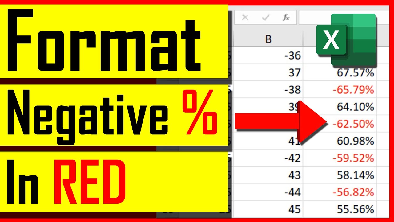
How To Format Negative Percentage In Red In Excel

08 Mar, 2021

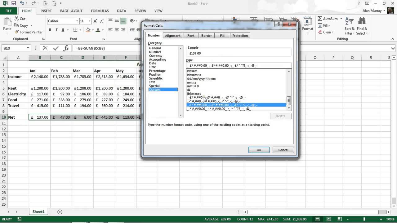
1 Select the cell or cells with the percent change number. Just above the list there is an area titles Type.

How To Create An Excel Custom Number Format Excelchat Excelchat

This provides you with the ultimate control over how the data is displayed.

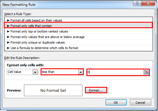
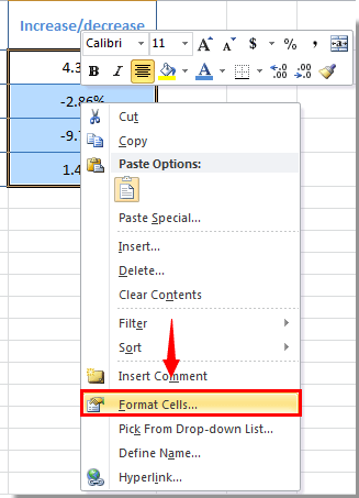
How to format negative percentage in red in excel. You can also select the cell and use hot keys Ctrl 1 to get to the number format window in step 3. In the New Formatting Rule dialog box please do as follows step by step. Click on Format Cells.

Create a Custom Negative Number Format. You can also create your own number formats in Excel. You may not realize that formatting numbers red vs black is conditional formatting although Excel does this a little differently.

The first method for highlighting negative values in red color is quite simple. In the Greater Than box enter 0 into the text box and then choose Custom Format. Cells that are formatted with the General format have no specific number format.

This option will display your negative number in red. Select the cells right click on the mouse. Then in the Styles group click on Conditional Formatting see screenshot at right and a palette of options appears.

In the Format Cells dialog. Finally click OK to close that screen and OK again to close Conditional Formatting. Add Brackets Minus Sign Mark Red All Negative PercentagesIn this Excel tutorial you ar.

Right click on the cell that you want to format. In Excel 2007 go to the Home tab and select the target cells. Create a conditional formatting for all negative percentage.

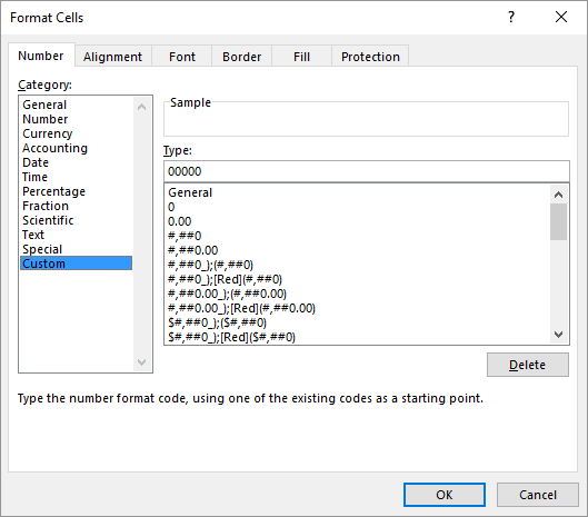
You will now see various custom formatting styles. You can also press Ctrl1. The format should resemble the following.

Show Negative Numbers in Bracket and in Red Color Select the cells which contain that list of the numbers as shown in the screenshot below. To select multiple cells hold down the Ctrl key as you. From the Number sub menu select Custom.

Right-click on the cell and select Format Cells. Choose custom and paste this in the dialog box for type. In the Number group click on the Format Cell dialog box launcher.

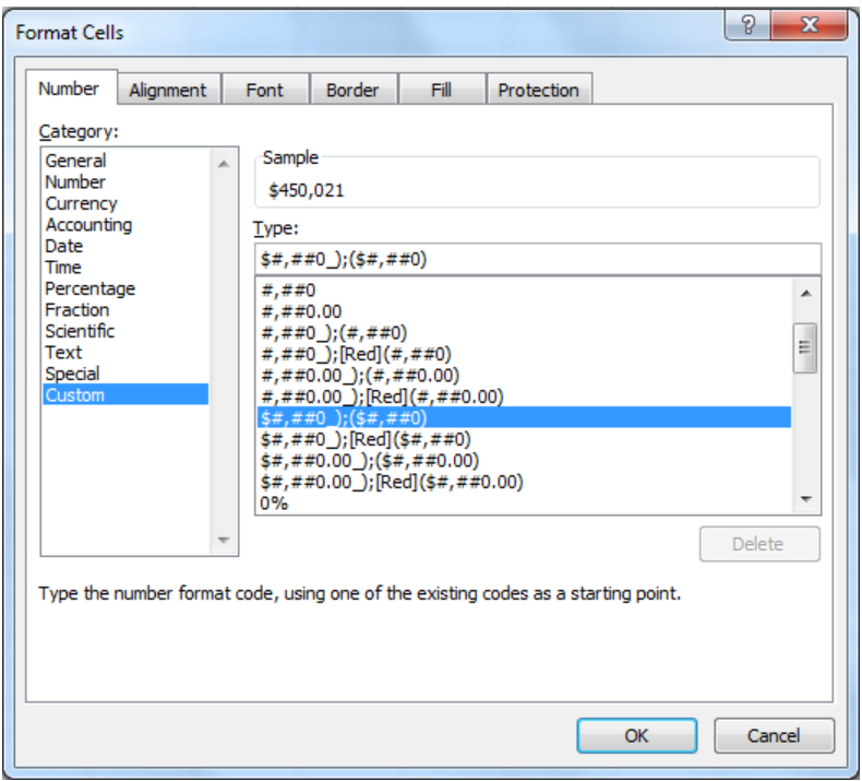
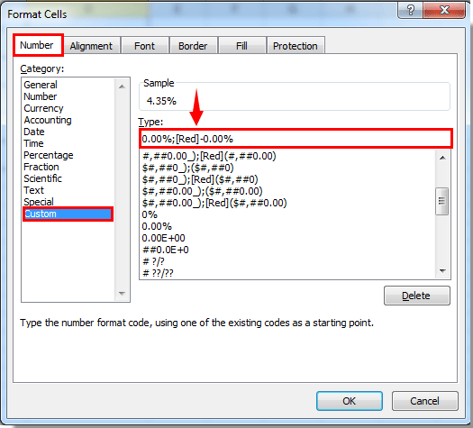
Select the cell or cells that contain negative percentages. Changing the number format to the predefined format for red negative numbers. If you want negative percentages to stand outfor example you want them to appear in redyou can create a custom number format Format Cells dialog box Number tab Custom category.

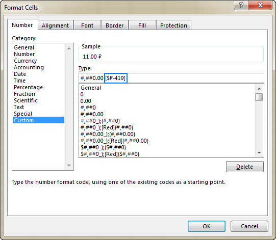
This lists all the ways a cell in Excel can be formatted. Excel provides a number format for highlighting negative values in red color. In the Format Cells box in the Category list click Custom.

Press the Font tab and select red see screenshot below. Select the cell range with negative percentage in current worksheet. Add Parenthesis to Negative Percentages.

Alternatively press Ctrl 1 on the keyboard. Here yoy can edit this formatting style. Add Brackets.

Click on Format Cells orPress Ctrl1 on the keyboard to open the Format Cells dialog box. At the bottom will be the Custom option. 2 From the drop down select More Number Formats at the bottom of the list.

Click Conditional Formatting New Rule under Home tab. To Format the Negative Numbers in Red Color with brackets. Select the numbers that you want to use and then click Home Conditional Formatting Greater Than see screenshot.

Hitting Ctrl 1 will launch the Format Cells menu. Start by right-clicking a cell or range of selected cells and then clicking the Format Cells command. Highlight the cells right-click format.

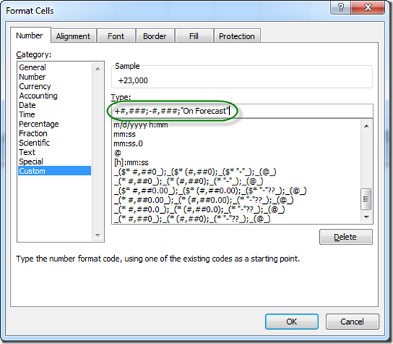
But for some reports negative numbers must be displayed with parenthesis. How to Mark Negative Percentage in Red in Microsoft ExcelIn this Excel tutorial you are about to learn two distinctive ways to mark or display negative per. In Excel to solve this task the Conditional Formatting also can do you a favor please do as this.

Select the Number tab and from Category select Number. Scroll down and you will see something like. Go to the Home Tab.

Negative numbers in Excel In Excel the basic way to format negative numbers is to use the Accounting number format. On the Home tab click Format Format Cells. In the Excel ribbon number section click the drop down that says General.

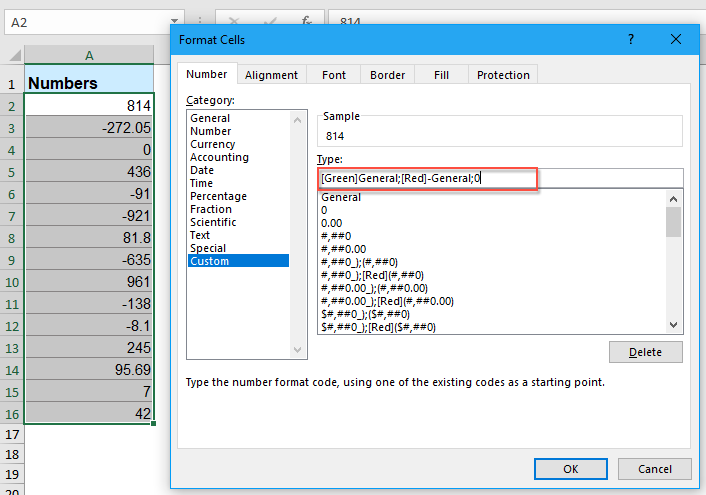
In the Type box enter the following format. Format the cell value red if negative and green if positive with Conditional Formatting function.

How To Mark Negative Percentage In Red In Microsoft Excel Youtube